Approached Theories
Basic RTA
- Table of Notation for Basic RTA
| Description | Symbol |
|---|---|
| Task | \(i\) |
| WC Response time | \(R_i^+\) |
| WC Execution time | \(C_i^+\) |
| Period | \(T_i\) |
| Frequency in Hz | \(f_m\) |
| Latency | \(L\) |
| Read Latency | \(L_{\uparrow m\to l}\) |
| Write Latency | \(L_{\downarrow m\to l}\) |
| Read labels | \(\mathcal{R}_i\) |
| Written Labels | \(\mathcal{W}_i\) |
| Label | \(\mathcal{L}\) |
| Label Size | \(\mathcal{S}\) |
Memory Access Cost
Memory access time is different depending on the target hardware. In this project, the memory access time is defined based on NVIDIA-TX2 platform. The equation for deriving this is referenced the WATERS19 projects namely CPU-GPU Response Time and Mapping Analysis for High-Performance Automotive Systems
\(L_{a,i}^+ = \sum_{x \in \mathcal{R}_i} \left( \left\lceil \frac {\mathcal{S}_x} {64} \right \rceil \right) \cdot \frac {L_{\uparrow m\to l}} {f_m} + \sum_{y \in \mathcal{W}_i} \left( \left \lceil \frac {\mathcal{S}_y} {64} \right \rceil \right) \cdot \frac {L_{\downarrow m\to l}} {f_m}\)
Here, the constant 64 is used as the baseline derived from the WATERS19 challenge description. \(ls\) denotes the label size and \(rl\) and \(wl\) define given read label and write label latencies specified in the given AMALTHEA model.
To find relevant methods, see CPU Task Execution Time.
Synchronous & Asynchronous Mechanism
In the provided AMALTHEA WATERS19 model, some of the tasks that are mapped to CPU trigger tasks mapped to GPU. In this case, the execution or response time can be different according to the offloading mechanism.
- Synchronous
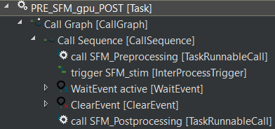
The triggering task triggers its target GPU task when it reaches InterProcessTrigger and actively waits until it receives the triggered task’s result after the response from the triggered GPU task. Then it finishes the remaining job.
- Asynchronous
The triggering task triggers its target GPU task when it reaches InterProcessTrigger and passively waits for the response from the triggered GPU task and finishes the remaining job.
During the passive waiting phase, other lower priority tasks can execute on the processor.
The asynchronous methodology described here can be modified according to the user’s interpretation.
This concept is used in two of the four execution cases introduced by a method, CPU Task Execution Time.
Response Time
The response time analysis approach implemented here is not only designed for Multi-core Systems but also for Heterogeneous Systems. Basically, the following classical response time analysis equation is used.
\(R_i = C_i + \sum_{j \in hp(i)} \left\lceil \frac {R_{i-1}} {T_j} \right\rceil C_j\)
The equation is based on RMS (Rate Monotonic Scheduling) which means that static priorities are assigned to tasks according to their period. A task with the shorter period results in a higher task priority. Here, \(R_i\) denotes the response time of task \(\tau_i\) and \(hp(i)\) is the set of tasks indexes (j) which have a priority higher than task i.
To find relevant methods, see Response Time Sum.
End-to-End Latency
The approach and its equations used here are referenced from a yet-unpublished paper, “Model-based Task Chain Latency and Blocking Analysis for Automotive Software” by the same authors who published CPU-GPU Response Time and Mapping Analysis for High-Performance Automotive Systems.
- Table of Notation for End-to-End Latency
| Symbol | Description |
|---|---|
| Task | \(\tau\) |
| Response time | \(R\) |
| Execution time | \(C\) |
| Period | \(T\) |
| Task chain | \(\gamma\) |
| Latency | \(\delta\) |
| implicit communication | \(\iota\) |
| LET communication | \(\lambda\) |
| Age latency | \(\alpha\) |
| Reaction latency | \(\rho\) |
| Reaction update | \(\upsilon\) |
Task Chain Reaction
The time between the task chain’s first task release to the earliest task response of the last task in the chain.
Task Chain Reaction (Implicit)
- Best-case Task-Chain Reaction (Implicit Communication Paradigm)
\(\delta_{\gamma,\rho,\iota} ^-=\sum_j R_{j}^- \text{ with } \tau_j \in \gamma\)
The best-case task chain reaction latency for implicit communication can be calculated by considering the sum of all task’s best case response times within task chain. Here, \(\gamma\) refers to a task chain, \(\rho\) corresponds the reaction latency, and \(\iota\) outlines that this latency considers the implicit communication paradigm.
- Worst-case Task-Chain Reaction (Implicit Communication Paradigm)
\(\delta_{\gamma,\rho,\iota}^+ = \sum_{j=0}^{j=|\gamma|-2} \left(2\cdot T_{j}\right) +R_{j = |\gamma|-1}^+ \text{ with } \tau_j \in \gamma\)
To find relevant methods, see Task Chain Reaction (Implicit Communication Paradigm).
Task Chain Reaction (LET)
- Best-case Task-Chain Reaction (Logical Execution Time)
\(\delta_{\gamma,\rho,\lambda} ^- = \sum_j T_{j} \text{ with } \tau_j \in \gamma\)
The best-case task chain reaction latency for LET communication is the sum of all task’s periods within task chain \(\gamma\).
- Worst-case Task-Chain Reaction (Logical Execution Time)
\(\delta_{\gamma,\rho, \lambda}^+= T_{j=0}+\sum_{j=1}^{j=|\gamma|-1} \left(2\cdot T_{j}\right) \text{ with } \tau_j \in \gamma\)
To find relevant methods, see Task Chain Reaction (Logical Execution Time Communication Paradigm).
Task Chain Age
The time a task chain result is initially available until the next task chain instance’s initial results are available. A task chain age latency equals the chain’s last (response) task age latency, i.e. \(\delta_{\gamma,\alpha} = \delta_{i,\alpha}\) with \(\tau_i\) being the last task of the task chain \(\gamma\), i.e. \(i=|\gamma|-1\).
- Best-case Task-Chain Age
\(\delta_{i, \alpha}^- = T_i - R_i^+ + R_i^-\)
- Worst-case Task-Chain Age
\(\delta_{i,\alpha}^+ = 2 \cdot T_i - R_i^- - (T_i - R_i^+) = T_i - R_i^- + R_i^+\)
To find relevant methods, see Task Chain Age.
Reaction Update
Due to the fact that tasks can have varying periods across the task chain, propagation between task chain entities can be over or under sampled such that a task X’s result (a) serves as an input for several subsequent task chain entity instances or (b) does not serve as an input at all due to the fact that the subsequent task can already work with newer results produced by X’s next instance.
Early Reaction
\(\delta_{\gamma, \rho 0, \iota}^+ = R_{\gamma0} + \sum_{j=0}^{j = |\gamma|-2} T_{j+1} + \min(T_{j+1}, \epsilon_j + R_{j+1})\)
\(\epsilon_j = 2\cdot T_{j} - R_{j} - T_{j+1} - \epsilon_{j-1}\)
\(\epsilon_{-1} = 0\)
To find relevant methods, see Task Chain Early Reaction.
Reaction Update
Accordingly, the reaction update is the subtraction of two consecutive task chains instances best case early reaction and worst case early reaction.
\(\delta_{\gamma, \upsilon, \iota}^+ = \max_{k} \left(T_{j=0} + \delta_{\gamma, \rho 0, \iota, k+1}^+ - \delta_{\gamma, \rho , \iota, k}^- \right)\)
Data Age
It describes the longest time some data version persists in memory. This is independent of task chains and simply depends on the period of entities writing a particular label (i.e. data).
- Best-case Data Age
\(\delta_{l,\alpha}^+ = \min_i \delta_{i,\alpha}^+\) with \(\tau_i\) being any task that accesses label \(l\).
- Worst-case Data Age
\(\delta_{l,\alpha}^- = \min_i \delta_{i,\alpha}^- %R_i^- + (T_i - R_i^+)\) with \(\tau_i\) being any task that accesses label \(l\).
To find relevant methods, see Data Age.